ML Crash Course Blog

A short crash-course on the fundamentals of Machine Learning.

Introduction to Machine Learning

This section provides a high-level overview of machine learning, establishing the core goal of generalization and introducing the main paradigms of learning. It sets the stage for understanding not just what ML is, but why it's structured the way it is. If you want to refresh your math fundamentals before diving into this click here - Math Fundamentals (RECOMMENDED)

1.1. What is Machine Learning?

At its core, Machine Learning is the science of getting computers to act without being explicitly programmed. Instead of writing a fixed set of rules, we provide algorithms with large amounts of data and let them learn the rules and patterns for themselves. The formal definition by Tom Mitchell provides a more structured view:

"A computer program is said to learn from experience E with respect to some class of tasks T and performance measure P, if its performance at tasks in T, as measured by P, improves with experience E."

Let's break this down with a real-world example: a spam filter.

  • Task (T): To classify emails as either "spam" or "not spam".
  • Experience (E): A massive dataset of emails, where each one has already been labeled by humans as spam or not spam.
  • Performance (P): The percentage of emails the program correctly classifies.

The ultimate goal is generalization: the ability of the model to perform accurately on new, unseen emails it has never encountered before, not just the ones it was trained on.

1.2. The Pillars of ML

Supervised Learning

Think of this as learning with a teacher or an answer key. The model is given a dataset where each data point is tagged with a correct label or output. The goal is to learn a mapping function that can predict the output for new, unseen data. It's like a student studying flashcards where one side is the question (input) and the other is the answer (label).

Unsupervised Learning

This is learning without an answer key. The model is given data without explicit labels and must find structure or patterns on its own. A common task is clustering, or grouping similar data points together. Imagine being given a box of mixed Lego bricks and you sort them into piles based on their shape and color without any instructions.

Self-Supervised Learning

This is a clever type of supervised learning where the labels are generated from the input data itself. For example, you could take a sentence, remove a word, and then train a model to predict that missing word. The "label" is the word you removed, but you didn't need a human to create it. This allows models to learn from vast amounts of unlabeled text or image data.

Reinforcement Learning

This is learning through trial and error, like training a pet. An "agent" (the model) learns to make decisions by performing actions in an "environment" to maximize a cumulative reward. It learns from the consequences of its actions, receiving positive rewards for good actions and penalties for bad ones.

1.3. The ML Workflow

Nearly every machine learning project follows a standard, iterative lifecycle. Understanding these steps is crucial for building effective models.

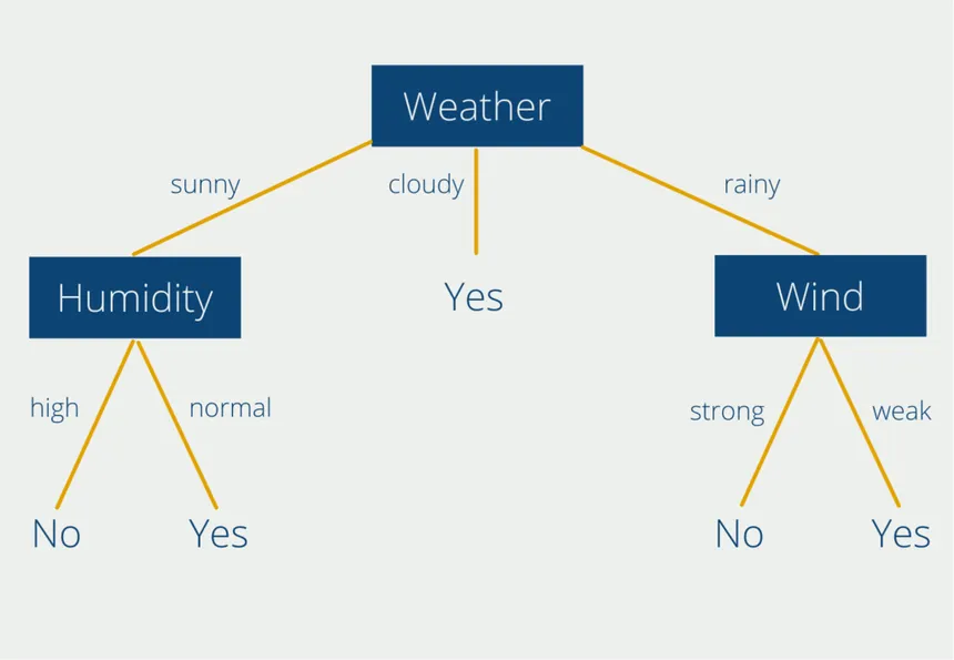
  1. Problem Framing: Define the objective. What question are you trying to answer? Is it a regression problem (predicting a number) or a classification problem (predicting a category)? What metric will define success?
  2. Data Collection & Preprocessing: Gather the necessary data. This is often the most time-consuming step, involving cleaning the data (handling missing values, outliers), feature engineering (creating new input signals), and scaling features to a common range.
  3. Model Selection & Training: Choose a suitable algorithm and feed it the prepared training data. The model learns the underlying patterns during this "training" phase.
  4. Evaluation: Assess the model's performance on a held-out test set—data it has never seen before. This gives an unbiased estimate of how it will perform in the real world.
  5. Hyperparameter Tuning: Adjust the model's settings (hyperparameters, like the 'k' in k-NN) to improve performance, often using a validation dataset to prevent overfitting to the test set.
  6. Deployment: Integrate the trained model into a production environment where it can make predictions on new, live data.

Supervised Learning - Regression

Regression models are used when the goal is to predict a continuous numerical value. This section focuses on the foundational algorithms for this task.

2.1. Linear Regression

Fits a "line of best fit" to the data. It models a linear relationship between input features (X) and a continuous target variable (y). For example, predicting a house's price based on its square footage.

ŷ = β₀ + β₁x₁ + ... + βₚxₚ

The Loss Function:

The model learns by minimizing the Mean Squared Error (MSE):

L(β) = (1/n) * Σ(yᵢ - ŷᵢ)²
  • yᵢ is the actual value for the i-th data point.
  • ŷᵢ is the model's predicted value.
  • n is the number of data points.
  • β is the vector of model parameters (the coefficients). The dimension of β is (p + 1) x 1, where 'p' is the number of features.

How it Learns: Finding the Parameters

There are two primary methods to find the optimal parameters (β) that minimize the MSE loss:

  1. Closed-Form Solution (Normal Equation): This is a direct mathematical formula that calculates the optimal parameters in one step: `β = (XᵀX)⁻¹Xᵀy`. It's efficient for smaller datasets but can be computationally expensive for datasets with a very large number of features.
  2. Gradient Descent: This is an iterative optimization algorithm. It starts with random parameter values and repeatedly adjusts them in the direction that most reduces the loss function, like walking downhill to find the bottom of a valley. For Linear Regression, the MSE loss function is convex, meaning it has only one global minimum. Therefore, gradient descent will always converge to the same optimal solution, regardless of the starting point.

Key Assumptions:

Linearity

The relationship between inputs and the output is linear. If the true relationship is curved (e.g., house price doesn't increase linearly with size forever), the model will be inherently inaccurate.

Independence

The errors (residuals) are independent. This means the error of one prediction is not influenced by the error of another. (Commonly violated in time-series data, where yesterday's stock price error affects today's).

Homoscedasticity

The errors have constant variance across all levels of the input features. A violation (heteroscedasticity) might mean the model is very accurate for cheap houses but highly inaccurate for expensive ones.

Normality of Errors

The errors are normally distributed. This is particularly important for statistical inference on the coefficients (e.g., determining if a feature is statistically significant).

2.2. Polynomial Regression

An extension of linear regression that can model non-linear relationships. It does this by adding polynomial terms (like x², x³, etc.) of the features as new features to the model.

ŷ = β₀ + β₁x₁ + β₂x₁² + ...

Why it's useful:

Many real-world relationships are not straight lines. For example, the relationship between a car's speed and its fuel efficiency is curved. Polynomial regression allows us to fit a more flexible, curved line to such data, leading to a more accurate model.

Supervised Learning - Classification

Classification models are used when the goal is to predict a discrete category or class label. This section covers the foundational algorithms for this task.

3.1. Logistic Regression

A baseline for classification that predicts the probability an input belongs to a class by passing a linear equation through a Sigmoid function. Example: Predicting if a loan application will be approved (Yes/No) based on income and credit score.

p̂ = 1 / (1 + e-(β₀ + β₁x₁ + ...))

How it Learns:

Unlike Linear Regression's MSE, Logistic Regression learns its coefficients by minimizing a different loss function called Log Loss (or Binary Cross-Entropy). This function penalizes confident but incorrect predictions more heavily, making it suitable for probabilistic classification.

L(β) = -(1/n) * Σ [yᵢ log(p̂ᵢ) + (1 - yᵢ) log(1 - p̂ᵢ)]

3.2. k-Nearest Neighbors (k-NN) Interactive Demo

A "lazy" algorithm that classifies a new point based on the majority vote of its 'k' closest neighbors. Example: Recommending a movie to a user based on the 'k' most similar users and what they liked.

How it Learns:

k-NN is a "lazy learner" because it doesn't have a distinct training phase. The "learning" consists of simply storing the entire training dataset in memory. All computation happens at prediction time, where it calculates the distance from a new point to every point in the training data to find its nearest neighbors.

Click on the plot to add a data point, then run knn to see which group it gets categorised into. Run it with different K values to see how that changes the grouping.

3.3. Support Vector Machines (SVMs)

A "maximum margin" classifier that finds the hyperplane that best separates the classes by maximizing the distance to the nearest points of any class (the support vectors).

How it Learns:

SVMs learn by solving a constrained optimization problem. The goal is to find the parameters (w, b) of the hyperplane that maximize the margin, subject to the constraint that all data points are correctly classified. This is a complex mathematical problem often solved using techniques like Quadratic Programming.

3.4. Decision Trees & Random Forests

A flowchart of "if-then-else" questions that splits the data into purer subgroups. Example: A bank using a decision tree to decide if a customer is eligible for a loan.

How it Learns:

The tree is built using a process called recursive partitioning. Starting with the entire dataset at the root node, the algorithm searches for the feature and threshold that create the "best" split—the one that results in the greatest reduction in impurity (e.g., using Gini Impurity or Information Gain). This process is repeated for each new node until a stopping criterion (like maximum depth) is met.

Decision tree example

Source: databasecamp.de

How Random Forests Improve on Decision Trees:

A single decision tree can easily overfit the training data. Random Forests improve upon this by using an ensemble method called bagging. It builds an entire "forest" of different decision trees, each trained on a random subset of the data and a random subset of the features. To make a prediction, it takes a majority vote from all the individual trees. This process averages out the errors of individual trees and creates a more robust model that is less prone to overfitting.

Unsupervised Learning

Unsupervised learning deals with unlabeled data, seeking to find hidden patterns or intrinsic structures. This section explores the two primary tasks: clustering data into groups and reducing dimensionality to simplify data.

4.1. K-Means Clustering Interactive Demo

A centroid-based algorithm that partitions data into 'k' clusters. Example: A marketing team using K-Means to segment customers into distinct groups (e.g., "high-spending," "budget-conscious") for targeted campaigns.

How it Learns:

K-Means uses an iterative algorithm called Expectation-Maximization (E-M). It begins by randomly placing 'k' centroids on the data plot. Then it repeats two steps until the centroids stop moving: 1) Assignment Step (E-step): Each data point is assigned to its nearest centroid. 2) Update Step (M-step): The centroids are recalculated as the mean (center) of all points assigned to them. This interactive demo visualizes this exact process.

Strengths & Weaknesses:

  • Strengths: Simple to understand, fast, and efficient on large datasets.
  • Weaknesses: The number of clusters 'k' must be specified beforehand, it's sensitive to the initial random placement of centroids, and it assumes clusters are spherical and evenly sized.

4.2. Principal Component Analysis (PCA)

A dimensionality reduction technique that transforms a large set of variables into a smaller one that still contains most of the information in the large set. Example: A geneticist might use PCA to reduce thousands of gene expression measurements into two or three "principal components" to visualize the main patterns of genetic variation in a population.

How it Works:

PCA is not an iterative learning algorithm but a mathematical transformation. It finds the directions of maximum variance in the data and projects the data onto a new, smaller-dimensional subspace. These new axes are the principal components.

  • Covariance Matrix (Σ): PCA starts by computing this matrix, which describes the variance of each feature and the covariance between pairs of features.
  • Eigenvectors & Eigenvalues: It then calculates the eigenvectors and eigenvalues of the covariance matrix. An eigenvector represents a direction (a principal component), and its corresponding eigenvalue indicates how much variance in the data lies along that direction.
  • By ranking the eigenvectors by their eigenvalues, PCA identifies the directions that capture the most information.

Model Training & Evaluation

Building a model is only half the battle; we must also rigorously evaluate its performance and understand its limitations. This section covers the crucial concepts of model validation, key performance metrics, and the fundamental Bias-Variance Tradeoff.

5.1. Evaluation Metrics

To evaluate a classification model, we use a Confusion Matrix to see where the model made correct and incorrect predictions. From this, we derive several key metrics:

  • True Positive (TP): The model correctly predicted the positive class.
  • False Positive (FP): The model incorrectly predicted the positive class.
  • True Negative (TN): The model correctly predicted the negative class.
  • False Negative (FN): The model incorrectly predicted the negative class.
  • Precision: Answers the question: "Of all the times the model predicted positive, how often was it right?" It's important when the cost of a false positive is high (e.g., a spam filter incorrectly flagging an important email).
    TP / (TP + FP)
  • Recall: Answers the question: "Of all the actual positive cases, how many did the model correctly identify?" It's important when the cost of a false negative is high (e.g., a medical test failing to detect a disease).
    TP / (TP + FN)
  • F1-Score: The harmonic mean of Precision and Recall, providing a single score that balances both metrics.
    2 * (Precision * Recall) / (Precision + Recall)
  • ROC/AUC: The ROC curve plots True Positive Rate vs. False Positive Rate. The AUC (Area Under the Curve) measures the entire area underneath the ROC curve. An AUC of 1.0 is a perfect classifier, while 0.5 is no better than random guessing.

    To evaluate a regression model:

    • Mean Absolute Error (MAE): The average of the absolute differences between the predicted and actual values.
      $$\frac{1}{n} \sum_{i=1}^{n} |y_i - \hat{y}_i|$$
    • Mean Squared Error (MSE): The average of the squared differences between the predicted and actual values.
      $$\frac{1}{n} \sum_{i=1}^{n} (y_i - \hat{y}_i)^2$$

    5.2. Cross-Validation

    A single train-test split can be misleading; the model's performance might be good or bad just by luck of the split. Cross-Validation provides a more robust estimate of performance. In k-fold cross-validation, the data is split into 'k' folds. The model is trained on k-1 folds and tested on the remaining fold. This process is repeated 'k' times, with each fold serving as the test set once. The performance scores are then averaged. This is crucial because it ensures the model's performance isn't a fluke, especially when data is limited.

    5.3. The Bias-Variance Tradeoff

    This is the central challenge in supervised learning. A simple model (low complexity) is underfit and has high bias (it's systematically wrong). A complex model (high complexity) is overfit and has high variance (it's too sensitive to the training data). The goal is to find the "sweet spot" of complexity that minimizes the total error.

    5.4. Regularization

    Regularization is a set of techniques used to prevent overfitting and thus improve the generalization of a model. It works by adding a penalty term to the model's loss function, which discourages the model from learning overly complex patterns by keeping the parameter values small.

    L1 (Lasso)

    The diamond-shaped constraint (left image) makes it likely the loss contours will touch at an axis, forcing a coefficient to exactly zero. This performs a type of automatic feature selection.

    L2 (Ridge)

    The circular constraint (right image) makes it unlikely the contours will touch exactly at an axis. Coefficients get smaller, but are rarely forced to zero.

    5.5. Hyperparameter Tuning for Slow Models

    When training time is very long, exhaustive methods like Grid Search are impractical. Better approaches include:

    • Random Search: Instead of trying every possible combination, Random Search samples a fixed number of random combinations from the hyperparameter space. It's often more efficient and can find very good parameters faster.
    • Bayesian Optimization: This is a more intelligent approach where the results from previous trials are used to inform which set of hyperparameters to try next. It builds a probabilistic model of the loss function and uses it to select the most promising parameters to evaluate, making it highly efficient for expensive models.

    Advanced Topics & Deep Learning

    This section introduces more advanced theoretical concepts and provides a glimpse into deep learning, the subfield of ML that powers many state-of-the-art applications.

    6.1. Feed-Forward Neural Network

    A model inspired by the brain, composed of interconnected "neurons" organized in layers. Each neuron takes in weighted inputs, applies an activation function, and passes its output to neurons in the next layer. By stacking these layers, the network can learn highly complex, non-linear patterns from the data, far beyond what simpler models can achieve.

    Input

    Hidden Layer

    Output

    6.2. How Neural Networks Learn

    Networks learn by minimizing a loss function. This is achieved through an optimization process involving two key algorithms:

    • Gradient Descent: An optimization algorithm that iteratively adjusts the model's parameters (weights and biases) to find the minimum of the loss function. The size of the adjustments is controlled by the Learning Rate (α).
    • Backpropagation: The algorithm used to efficiently calculate the gradient (the direction of steepest ascent) of the loss function with respect to every weight and bias in the network. It works by propagating the error backward from the output layer to the input layer.

    1. Forward Pass →

    Input data flows through the network to produce an output (prediction).

    2. Compute Loss

    Compare the prediction to the true label to calculate the error.

    3. Backward Pass (Backpropagation) ←

    Calculate the gradient of the loss with respect to each parameter.

    4. Update Parameters

    Adjust weights and biases using Gradient Descent to reduce the loss.

    6.3. Foundational Concepts - Bayes' Theorem

    Bayes' Theorem is a mathematical way to update your beliefs based on new evidence. It starts with a prior belief (what you think is true initially) and combines it with the likelihood of seeing new evidence, resulting in an updated, more informed posterior belief. In simple terms: Initial Belief + New Evidence = Updated Belief.

    • P(A) - Prior: Your initial belief about the hypothesis A before seeing any evidence. It's the "base rate." Example: The general probability that any given email is spam. If 20% of all emails are spam, then the prior:
      $$P(A = \text{Spam}) = 0.2$$
    • P(B) - Evidence or Marginal Likelihood: The total probability of observing the evidence B under all possible hypotheses. It acts as a normalization constant. Example: The overall probability that any email contains the word "lottery". This is the sum of the probability it appears in spam and the probability it appears in non-spam:
      $$P(\text{"lottery"} \mid \text{Spam}) \, P(\text{Spam}) + P(\text{"lottery"} \mid \text{Not Spam}) \, P(\text{Not Spam})$$
    • P(B|A) - Likelihood: The probability of observing evidence B if hypothesis A is true. Example: The probability that an email contains the word "lottery" given that it is spam. Since spammers use this word often, the likelihood might be high, say 0.7:
      $$P(B = \text{"lottery"} \mid A = \text{Spam}) = 0.7$$
    • P(A|B) - Posterior: Your updated belief about the hypothesis A after considering the evidence B. This is the result you want to calculate. Example: The probability that an email is spam given that it contains the word "lottery". Bayes' theorem lets you calculate this updated, more informed probability.
      $$P(A \mid B) = \frac{P(B \mid A) \, P(A)}{P(B)}$$

    6.4. Generative vs. Discriminative Models

    Discriminative Models

    Learn the decision boundary between classes. They model the conditional probability P(Y∣X). They directly learn to distinguish between classes Their goal is to distinguish between categories. They essentially learn to answer the question: "Given this input, what is the probability of this label?"

    Examples: Logistic Regression, SVMs, standard Neural Networks.

    Generative Models

    Learn the underlying distribution of the data for each class. They model the joint probability P(X,Y). Because they learn how the data is generated, they can be used to create new, synthetic data points. They learn what the data for each category looks like.

    Examples: Generative Adversarial Networks (GANs), Variational Auto-Encoders (VAEs).

    Machine Learning Algorithms Comparison

    Algorithm Type Use Case Time Complexity Space Complexity Pros Cons
    Supervised Learning
    Linear Regression Regression Predict numerical values O(n * d) O(d) Simple, interpretable Assumes linear relationship, sensitive to outliers
    Logistic Regression Classification Binary/multi-class classification O(n * d) O(d) Fast, interpretable, probabilistic output Limited to linear decision boundaries
    Decision Trees Classification & Regression Classification, regression, feature importance O(n * d * log n) O(n) Interpretable, handles nonlinear data Prone to overfitting, unstable
    Random Forest Ensemble Classification, regression O(t * n * d * log n) O(t * n) Reduces overfitting, robust Less interpretable, slower for many trees
    Support Vector Machine (SVM) Classification High-dimensional classification tasks O(n² * d) to O(n³) O(n * d) Effective in high dimensions Slow on large datasets, kernel choice matters
    K-Nearest Neighbors (KNN) Classification & Regression Classification, recommendation systems O(n * d) per query O(n * d) Simple, no training phase Slow for large datasets, sensitive to irrelevant features
    Gradient Boosting (XGBoost, LightGBM) Ensemble High-performance regression and classification O(t * n * log n * d) O(n * d) High accuracy, handles missing values Training is slower, prone to overfitting if not tuned
    Neural Networks (Deep Learning) Regression & Classification Image recognition, NLP, complex patterns O(n * d * L) O(n * d + parameters) Flexible, handles complex data Black-box, needs large data, computationally expensive
    Unsupervised Learning
    k-Means Clustering Grouping, customer segmentation O(n * k * i * d) O(n * d) Fast, simple, scalable Needs predefined k, sensitive to initialization
    Hierarchical Clustering Clustering Grouping, dendrogram analysis O(n³) O(n²) No need for predefined clusters, dendrogram visual Very slow on large datasets
    Principal Component Analysis (PCA) Dimensionality Reduction Reducing dimensionality, visualization O(n * d² + d³) O(d²) Reduces noise, speeds up other ML algorithms Linear method, may lose interpretability